Conditional formatting in Google Sheets changes the appearance of cells automatically when a rule is true. You can highlight overdue tasks, flag duplicate IDs, show high and low values, or color an entire row based on its status. The feature changes the display, not the underlying data.
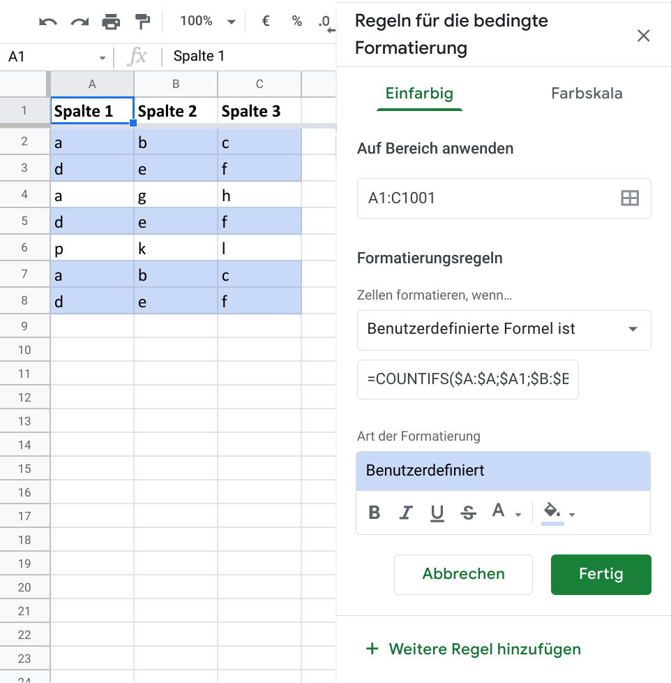
How to add conditional formatting in Google Sheets
- Open a spreadsheet and select the cells you want to format, such as
A2:D100. - Choose Format → Conditional formatting from the menu.
- In the sidebar, check the Apply to range field.
- Under Format cells if, choose a condition such as Text is exactly, Greater than, or Custom formula is.
- Enter the value or formula, choose a fill or text color, and select Done.
- Change a source cell to confirm that the rule updates as expected.
Conditional formatting rules can overlap. If your results look inconsistent, review every rule affecting the selected range and simplify conflicting conditions.
Seven practical conditional formatting examples
| Goal | Apply to range | Condition |
|---|---|---|
| Highlight tasks marked Done | D2:D100 | Text is exactly: Done |
| Flag amounts over $1,000 | C2:C100 | Greater than: 1000 |
| Highlight overdue task rows | A2:D100 | =AND($B2<TODAY(),$D2<>"Done",$B2<>"") |
| Find duplicate IDs | A2:A100 | =AND(A2<>"",COUNTIF($A$2:$A$100,A2)>1) |
| Highlight an entire completed row | A2:D100 | =$D2="Done" |
| Mark blank required cells | B2:B100 | Is empty |
| Color high-to-low values | C2:C100 | Color scale |
These examples assume column A stores IDs, B stores due dates, C stores amounts and D stores status. Adapt the column letters to your own sheet. Some locales require semicolons instead of commas in formulas.
Example 1: highlight a whole row when status is Done
Suppose each task occupies columns A through D, and its status is in D. Select A2:D100, open conditional formatting, choose Custom formula is, and enter:
=$D2="Done"The dollar sign before D locks the status column while the row number remains relative. This lets Google Sheets evaluate D2 for the first row, D3 for the second, and so on. Without the dollar sign, the rule could shift its check into columns E, F and beyond as it colors cells across the row.
Choose a light green fill or another accessible color. Test the rule by changing D2 to Done, then back to In progress.
Example 2: highlight overdue tasks but not completed ones
Assume due dates are in B and task status is in D. Select A2:D100 and enter this custom formula:
=AND($B2<TODAY(),$D2<>"Done",$B2<>"")It checks three things: the date is earlier than today, the status is not Done, and the due-date cell is not empty. The last condition prevents blank dates from being treated like old date serial values.
Important: The values in column B must be actual dates, not strings that merely look like dates. If the rule does not trigger, check the cell format and how the dates were imported.
Example 3: find duplicates in a list
Select A2:A100 and use:
=AND(A2<>"",COUNTIF($A$2:$A$100,A2)>1)COUNTIF counts how often the current cell’s value appears in the entire fixed range. The rule highlights entries that occur more than once, while the nonblank check prevents empty cells from being colored. It does not delete duplicates; it only makes them easier to review.
For duplicate detection across two columns together, a helper column that combines the two fields may be easier to audit than a complex formatting rule.
Example 4: flag sales above a target
Select the revenue cells, such as C2:C100. Choose Greater than and enter 1000. Any numeric amount above the threshold is highlighted. If the threshold should change often, put it in F1 and use a custom formula instead:
=C2>$F$1Now changing F1 updates the highlighting across the range. Keep the comparison value numeric, not a text string containing a currency symbol.
Example 5: use color scales for performance
Select a numeric range, then open the Color scale tab in the conditional formatting sidebar. Choose a gradient and set minimum, midpoint or maximum values when needed. A scale is useful for comparing values across a table, but it can exaggerate differences when the dataset has extreme outliers. Show the actual numbers alongside the colors.
Example 6: highlight weekends in a calendar
If real dates are in column A, select A2:D100 and use:
=AND(ISNUMBER($A2),WEEKDAY($A2,2)>5)With the second WEEKDAY argument set to 2, Monday is 1 and Sunday is 7. Values greater than 5 are Saturday and Sunday. The ISNUMBER check avoids formatting blank or invalid date cells.
Example 7: highlight rows containing a keyword
If column C contains notes, select A2:D100 and use:
=ISNUMBER(SEARCH("urgent",$C2))SEARCH is case-insensitive and returns the position of the text when found. ISNUMBER turns a successful match into TRUE, while a missing match becomes FALSE. This highlights rows whose notes contain the word urgent anywhere in the text. If you need to match only a full word, a carefully constructed REGEXMATCH rule may be more appropriate.
How to edit or delete a conditional formatting rule
- Select a cell covered by the rule.
- Choose Format → Conditional formatting.
- In the sidebar, click the existing rule to edit its range, condition or appearance.
- To remove a rule, use its delete control. Removing the rule does not erase the spreadsheet’s values.
If a rule appears to be missing, check whether it applies to a different range. Multiple similar rules may have been created when rows or sheets were copied.
Conditional formatting not working? Check these causes
| Symptom | Likely cause | Fix |
|---|---|---|
| Only the first row changes | Wrong relative or absolute references | Check the dollar signs and the rule’s starting row |
| Dates do not highlight | Dates stored as text | Convert to real date values |
| Rule affects unrelated cells | Apply-to range too broad | Set the exact range |
| Duplicate rule highlights blanks | Missing nonblank condition | Add A2<>"" |
| Formula parse error | Wrong separators, quotes or parentheses | Check syntax and spreadsheet locale |
| Colors look unexpected | Overlapping rules | Review and simplify the rule list |
Frequently asked questions
Can conditional formatting color an entire row?
Yes. Apply a custom formula to the entire row range and lock the column used for the condition, such as =$D2="Done".
Does conditional formatting change cell values?
No. It changes appearance based on conditions. Use formulas or editing tools if you need to change the data itself.
Can I use a formula in conditional formatting?
Yes. Choose Custom formula is and enter a formula that evaluates to TRUE or FALSE for the first cell in the applied range.
Can I highlight duplicate values automatically?
Yes. Use a COUNTIF-based custom formula. The formatting updates as the list changes, but it does not remove duplicate rows.
Related guides and documentation
For functions used in these rules, see our Google Sheets formulas guide. Google’s official conditional formatting help covers additional examples and interface details. Test a rule on a small range before applying it to an entire business workbook.

Other Articles

Google Sheets Pivot Table Tutorial: Summarize Sales and Group Data
Minimize Window Shortcut on Windows 11 and 10: One, All and Restore